import random
import matplotlib.pyplot as plt
import matplotlib.animation as animation
import os
# 作業ディレクトリの指定。自分の好きなところに設定してください。
os.chdir("../images")
# AND素子のパーセプトロンの定義
def _and_(x, y, coe_x, coe_y, intercept):
return 1 if(coe_x*x + coe_y*y + intercept > 0) else 0
# 同じ要素が続いているかどうかの判定
def conse(ps):
result = [1]
for i in range(1, len(ps)):
result.append(0 if (ps[i-1] == ps[i]) else 1)
return result
# x,yの二変数関数からxの一変数関数への変換
def linear_func(x, coe_x, coe_y, intercept):
return (-1*coe_x*x - intercept)/coe_y
coe_x = random.random()
coe_y = random.random()
intercept = random.random()
LEARNING_RATE = 0.01
LIMIT = 1000
params = {"coe_x":[coe_x], "coe_y":[coe_y], "intercept":[intercept]}
# 学習
for i in range(LIMIT):
x = random.randint(0, 1)
y = random.randint(0, 1)
if(_and_(x, y, coe_x, coe_y, intercept)):
if not x or not y: # x,y = ?,0 or 0,?
intercept -= LEARNING_RATE
if not x and y: # x,y = 0,1
coe_y -= LEARNING_RATE
if x and not y: # x,y = 1,0
coe_x -= LEARNING_RATE
else:
if x and y:
coe_x += LEARNING_RATE
coe_y += LEARNING_RATE
intercept += LEARNING_RATE
params["coe_x"].append(coe_x)
params["coe_y"].append(coe_y)
params["intercept"].append(intercept)
# グラフに描画する配列の定義
params_shaped = {"coe_x":[], "coe_y":[], "intercept":[]}
coe_x_conse = conse(params["coe_x"])
coe_y_conse = conse(params["coe_y"])
coe_i_conse = conse(params["intercept"])
# 重複する要素を排除して先程の配列に格納
for i in range(len(coe_i_conse)):
if (coe_x_conse[i] or coe_y_conse[i] or coe_i_conse[i]):
params_shaped["coe_x"].append(params["coe_x"][i])
params_shaped["coe_y"].append(params["coe_y"][i])
params_shaped["intercept"].append(params["intercept"][i])
# 結果の出力
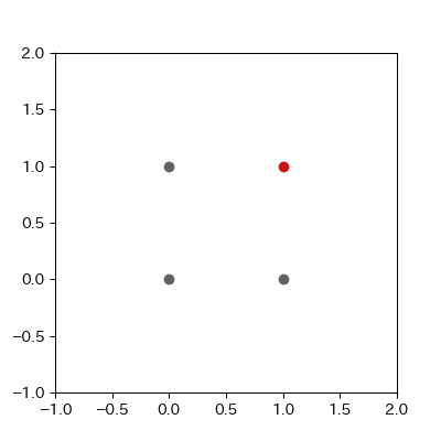
print(f"0 \u2227 0 = {_and_(0, 0, coe_x, coe_y, intercept)}")
print(f"1 \u2227 0 = {_and_(1, 0, coe_x, coe_y, intercept)}")
print(f"0 \u2227 1 = {_and_(0, 1, coe_x, coe_y, intercept)}")
print(f"1 \u2227 1 = {_and_(1, 1, coe_x, coe_y, intercept)}")
# グラフの描画領域の定義
fig = plt.figure(figsize=(4, 4))
ax = fig.add_subplot(111)
plt.xlim(-1,2)
plt.ylim(-1,2)
images = []
xs, ys = [], []
xs2, ys2 = [], []
# グラフの描画
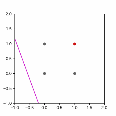
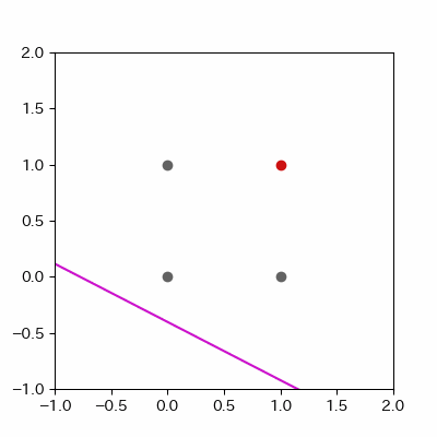
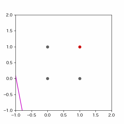
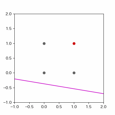
for p in range(len(params_shaped["intercept"])):
image = ax.plot([-1, 2],
[linear_func(-1, params_shaped["coe_x"][p], params_shaped["coe_y"][p], params_shaped["intercept"][p]),
linear_func(2, params_shaped["coe_x"][p], params_shaped["coe_y"][p], params_shaped["intercept"][p])],
c="#cc11cc")
xs.append(1)
ys.append(1)
point = ax.scatter(xs, ys, c="#cc1111")
xs2.append([0, 1, 0])
ys2.append([0, 0, 1])
point2 = ax.scatter(xs2, ys2, c="#616161")
images.append(image + [point] + [point2])
ADD_PLOT = 10
LEN_PARAMS = len(params_shaped["intercept"])-1
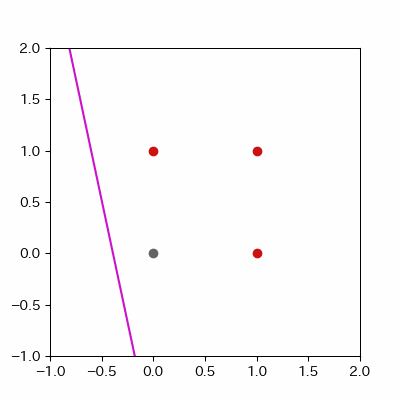
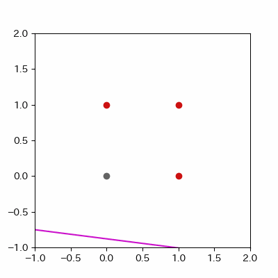
for a in range(ADD_PLOT):
image = ax.plot([-1, 2],
[linear_func(-1, params_shaped["coe_x"][LEN_PARAMS], params_shaped["coe_y"][LEN_PARAMS], params_shaped["intercept"][LEN_PARAMS]),
linear_func(2, params_shaped["coe_x"][LEN_PARAMS], params_shaped["coe_y"][LEN_PARAMS], params_shaped["intercept"][LEN_PARAMS])],
c="#ff1111")
xs.append(1)
ys.append(1)
point = ax.scatter(xs, ys, c="#cc1111")
xs2.append([0, 1, 0])
ys2.append([0, 0, 1])
point2 = ax.scatter(xs2, ys2, c="#616161")
images.append(image + [point] + [point2])
anime = animation.ArtistAnimation(fig, images, interval=100, repeat_delay=100)
anime.save("and_learn.gif", writer="pillow")
plt.show()